A factory pays for electricity from the grid at a price that changes every hour
(German day-ahead prices — they can even go negative).
It has three things it cannot control:
Industrial load — fixed demand it must serve
Solar PV — ~131 kW peak, weather-driven
Grid price — set by the market
…and one thing it can: a 1600 kWh battery. Charge it when power is
cheap, discharge when expensive → shift demand in time → lower the bill.
That decision is the agent's whole job.
💡 The core idea
Buy low, store it, use it when prices are high.
🔋 ➜ 💰
"Price arbitrage" with a battery
2 · System architecture
P_grid = P_load − P_PV + P_battery · the agent commands only the
green flow; the grid draw is whatever balances the bus.
3 · How the Deep-RL agent learns
No labelled data — the agent learns by trial and error from a reward signal, in a loop:
State (80 numbers): battery charge, time, current & past 24 h of
price and load, plus the next 24 h of known day-ahead prices.
Action: one of 21 battery power levels, −200 → +200 kW.
DQN = a neural net that scores every action; a "Double + Dueling" design plus
experience replay make it stable. Train 5 seeds, report the average.
4 · The dashboard — what's on it
One interactive page per agent. It replays the trained policy over the held-out
Oct–Dec test set and draws everything from the real step-by-step results:
KPI cards + banner
The 5-seed validated headline: saving, gap to optimum, preserved peak.
▶ Day player
Animate any test day step-by-step with a live "what's happening now" narration.
4 charts
The grid · the agent's decisions · the context · the cumulative cost. (Next slides →)
The next four slides explain each chart and, importantly,
what its X-axis and Y-axis mean.
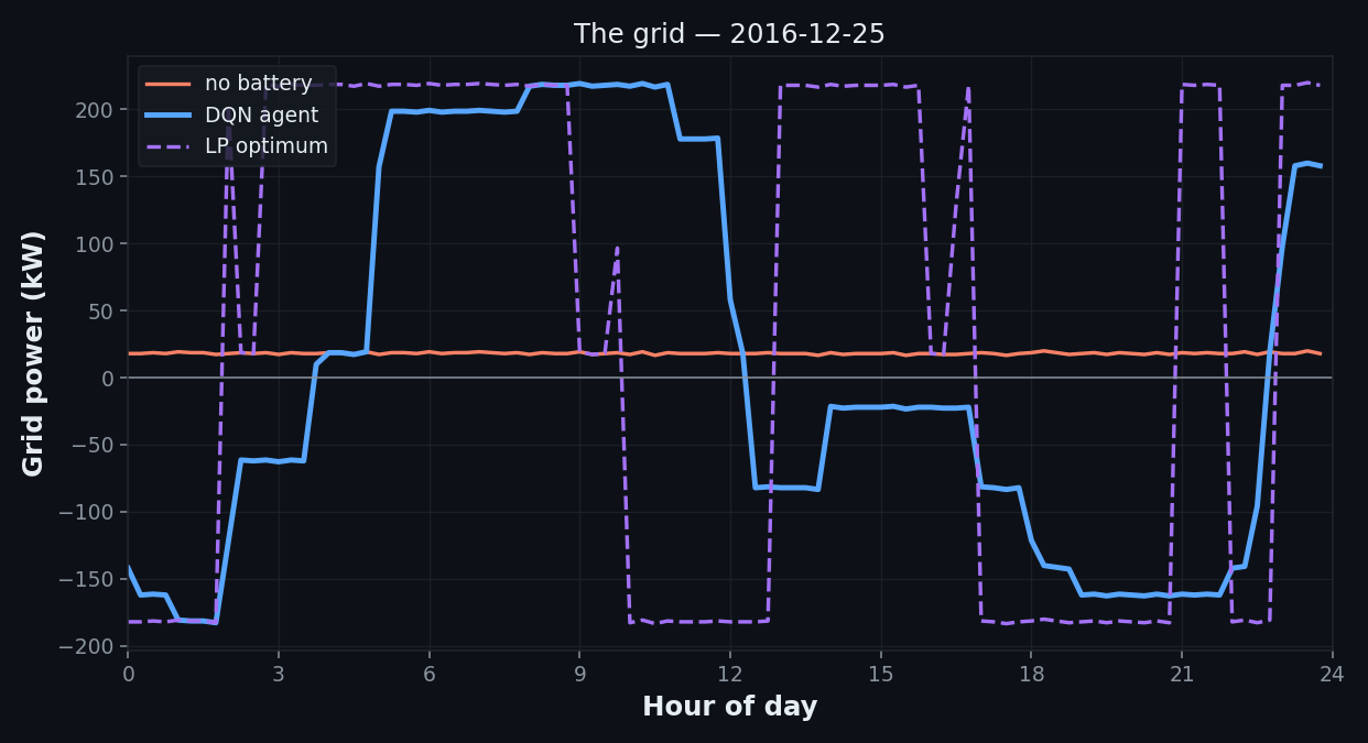
Read it as: the agent (blue) drops during expensive
hours and rises when cheap — hugging the LP optimum (purple dashed).
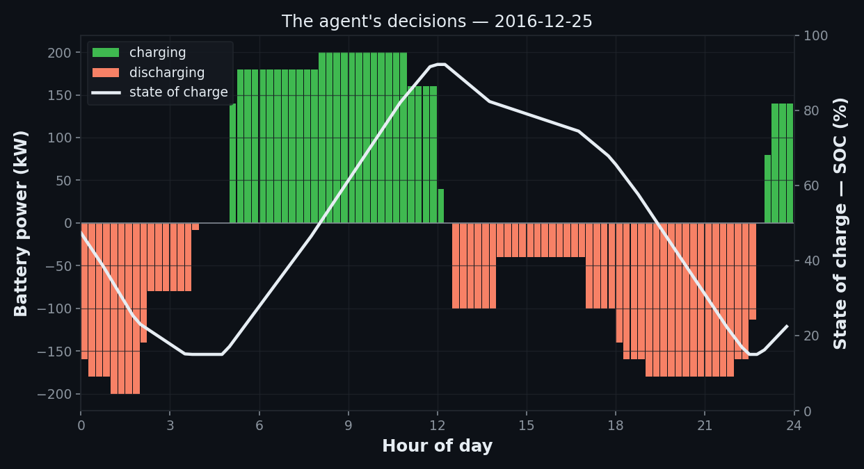
Chart 2 · The agent's decisions — battery power & charge
◀▶ X-axis
Hour of day
0 → 24 h (15-min steps)
▲▼ Left Y-axis
Battery power (kW)
+ green = charging · − orange = discharging
▲▼ Right Y-axis
State of charge — SOC (%)
0–100% · how full the battery is (white line)
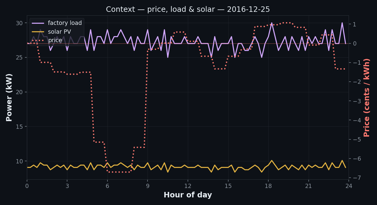
Chart 3 · Context — what drives the decision
◀▶ X-axis
Hour of day
0 → 24 h (15-min steps)
▲▼ Left Y-axis
Power (kW)
factory load & solar generation
▲▼ Right Y-axis
Price (cents / kWh)
can go < 0 — negative prices pay you to consume
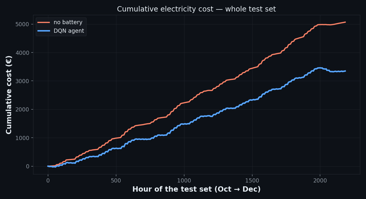
Chart 4 · Cumulative cost — the whole test set
◀▶ X-axis
Hour of the test set
the full Oct → Dec period, left → right
▲▼ Y-axis
Cumulative cost (€)
total euros spent so far
Read it as: the widening gap between the two
lines is the money the agent saves over the quarter.
5 · What we compare against
⊘ No-battery baseline
The factory with solar but no battery, no control. The bill to beat —
the upper bound on cost.
◆ Perfect-foresight LP
A solver told the whole day in advance → the cheapest schedule
physically possible. The target no controller can beat.
The agent sits between them:
32.9% below the baseline, only 8.0% above the optimum —
with no future knowledge beyond published day-ahead prices.
6 · The result (validated across 5 seeds)
Cost vs no-battery
−32.9%
€5069 → €3401 ± 117
Gap to LP optimum
8.0%
near-perfect
Grid peak
253 kW
≈ 250 baseline · preserved
On days it had never seen, the agent learned to cut the
electricity bill by about a third — landing within single digits of the perfect-foresight optimum,
without making the grid peak worse.